Updated: July 31, 2019

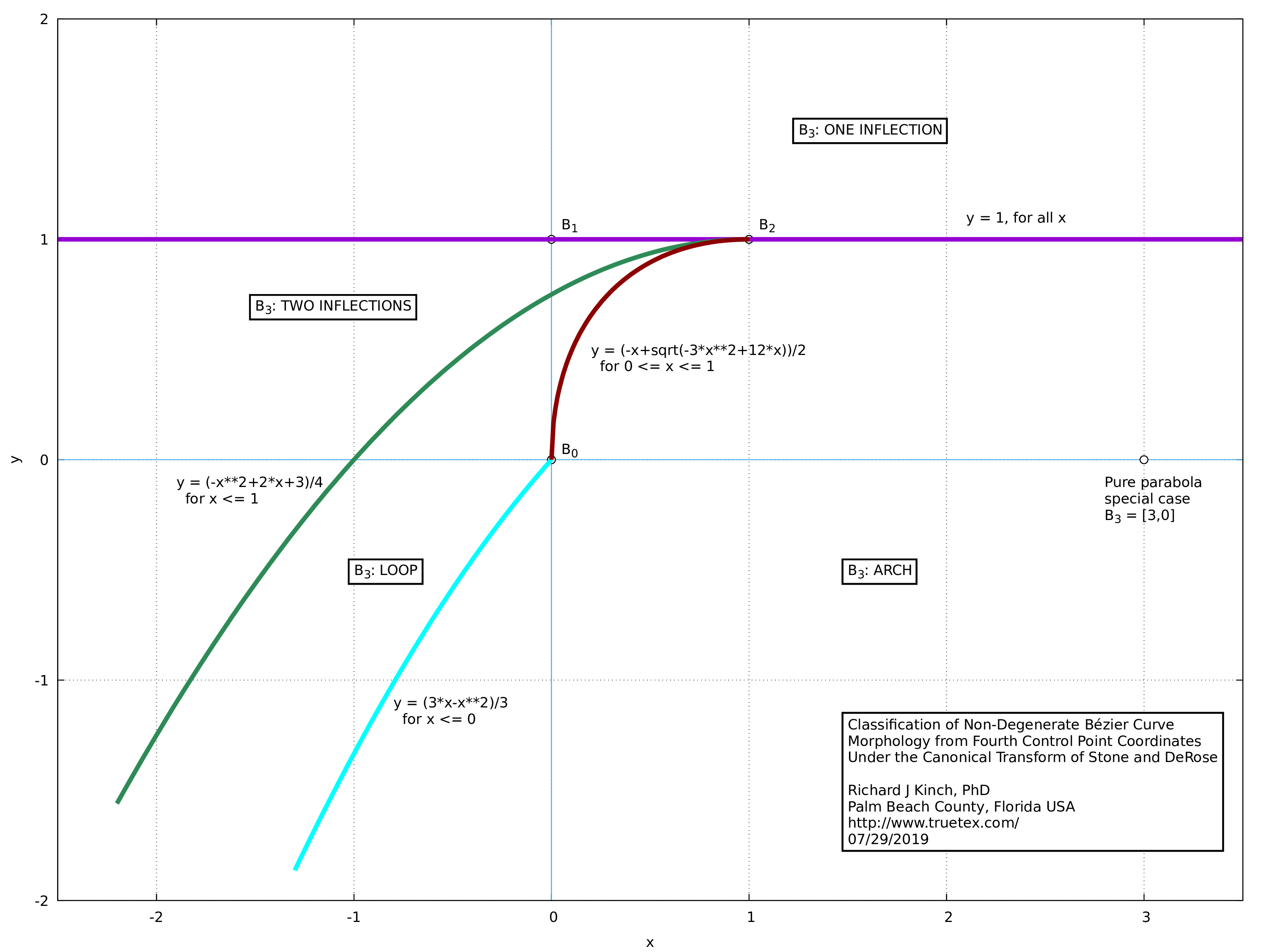
The plot (PDF version) and sample code below give my enhanced summary of how to classify the "motif" of Bézier curves based on the canonical transformation developed by Stone and DeRose in their paper, "A Geometric Characterization of Parametric Cubic Curves" (ACM Transactions on Graphics, Vol. 8, No. 3, July 1989). That paper presents the same plot, but is hard to interpret since it is poorly rendered in the online copy available on the Web. The paper also omits the explicit formulas and combinatoric logic necessary for computing and testing the region boundaries, which I have solved and incorporated into my version below. The Xerox PARC Technical Note which supposedly gave such details seems to be no longer available.

By the term "motif", I mean one of the four possible morphological forms of a non-degenerate curve. These four possibilities are: arch, loop, one inflection, or two inflections. The degenerate cases occur when the first two points, or the second and third points, are coincident.

Here is a code snippet (in AWK) which illustrates the necessary logic and math to implement the test, given that one has performed the transform and knows the B₃ coordinates:

# Analyzes the canonical-form fourth control point to detect the "motif" of k0--k1,
#   per Stone and DeRose.  Possible return values:
#
#       "A"     Arch
#       "L"     Loop
#       "1"     Single inflection
#       "2"     Double inflection
#       "D"     Degenerate (various coincidences or colinearities of control points
#                 which prevents the canonical transform)
#
# The region boundaries are the functions:
#   Explicit single inflection boundary: y > 1
#   Implicit cusp line: x^2 - 2x + 4y - 3 = 0
#       Explicit: y = (-x^2+2x+3)/4
#   Implicit loop line: x^2 - 3x + 3y = 0, for x < 0, y < 0
#       Explicit: y = (3x-x^2)/3
#   Implicit loop line: x^2 + y^2 +xy - 3x = 0, for 0 <= x < 1, 0 <= y < 1
#       Explicit: y = (-x+sqrt(-3x^2+12x))/2 [as the relevant quadratic formula solution]
#
function bezier_motif(k0,k1,
        b3,yhi,ylo) {
  if (bezier_canon(b3,k0,k1)) {
    if (b3[Y]>1) return "1"				# Region: y > 1
    else if (b3[X]>=1) return "A"                       # Region: x >= 1, y < 1
    else if (b3[X]>=0) {                                # Region: 1 > x >= 0, y < 1
      ylo = (-b3[X]+sqrt(-3*b3[X]^2+12*b3[X]))/2
      yhi = (-b3[X]^2+2*b3[X]+3)/4
      if (b3[Y]<ylo) return "A"                         # Region: below curve
      else if (b3[Y]<=yhi) return "L"                   # Region: between curves
      else return "2"                                   # Region: above curves but below y=1
      }
    # Region: x < 0, y < 1
    else {
      ylo = (3*b3[X]-b3[X]^2)/3
      yhi = (-b3[X]^2+2*b3[X]+3)/4
      if (b3[Y]<ylo) return "A"                         # Region: below curve
      else if (b3[Y]<=yhi) return "L"                   # Region: between curves
      else return "2"                                   # Region: above curves but below y=1
      }
    }
  else return "D"                                       # No canonical region
  }

Here is the code I use to compute the canonical transform point B₃, given the two input knots k₀ and k₁ of the curve. The code safely tests for degenerate cases and signals that occurence.

function bezier_canon(b3,k0,k1,
        b0,b1,b2,
        theta,factor) {
  # Local vector copies of the curve control points as b0..b3
  b0[X] = k0[BX] ; b0[Y] = k0[BY]
  b1[X] = k0[BOX] ; b1[Y] = k0[BOY]
  b2[X] = k1[BIX] ; b2[Y] = k1[BIY]
  b3[X] = k1[BX] ; b3[Y] = k1[BY]
  # Translate all to b0 = [0,0]
  itranslate(b1,b0)
  itranslate(b2,b0)
  itranslate(b3,b0)
  vset(b0,0,0)
  # Rotate b1..b3 to b1 = [0,+]
  theta = 90*DEG - knot_oa(k0)
  rotate(b1,theta)
  rotate(b2,theta)
  rotate(b3,theta)
  # Scale b2..b3 in Y to b1 = [0,1]
  if (b1[Y]==0) return 0 # degenerate b1
  factor = 1/b1[Y]
  vscale(b2,factor)
  vscale(b3,factor)
  vset(b1,0,1)
  # Scale b2..b3 in X to b2 = [1,y]
  if (b2[X]==0) return 0 # degenerate b2 X
  factor = 1/b2[X]
  b3[X] *= factor
  b2[X] = 1
  # Shear (y' = y + kx) b2..b3 to b2 = [1,1]
  factor = 1 - b2[Y]
  b3[Y] = b3[Y] + factor*b3[X]
  b2[Y] = 1
  return 1
  }