Consider just the "simple" case, where two Bezier curves intersect at singular point(s). The problem is to find the singular minima (or zeroes) of an N-dimensional non-linear distance function given two N-dimensional Bezier curves. This is the sort of problem about which Press et al. state, "There are no good, general methods for solving systems of more than one nonlinear equation. ... there never will be any good, general methods." [1] We will illustrate with some two-dimensional examples.
Here are two "normal" 2D cubic Bezier curves, each a two-dimensional function z(t) for t = [0,1]. (Parameter t is often spoken of as the "time" on the curve.) The curves are "normal" in the sense that they have no inflections or horizontal or vertical tangents. Nevertheless, the two curves intertwine such that they intersect in 4 singular locations. Straight line segments join each end of one curve to an end of the other curve, forming a closed path. One curve starts with its parameter t = 0 at the top left and runs to the bottom right at t = 1; the other curve runs in an opposite direction from bottom right at t = 0 to the top left at t = 1. Arrowheads indicate the direction of advancing time, dots indicate the endpoints (knots), and the dashed lines terminating in "x" marks indicate the control points. (The curves have been sectioned here for the intersection points, so that the control points shown do not reflect the original, unintersected curves.)
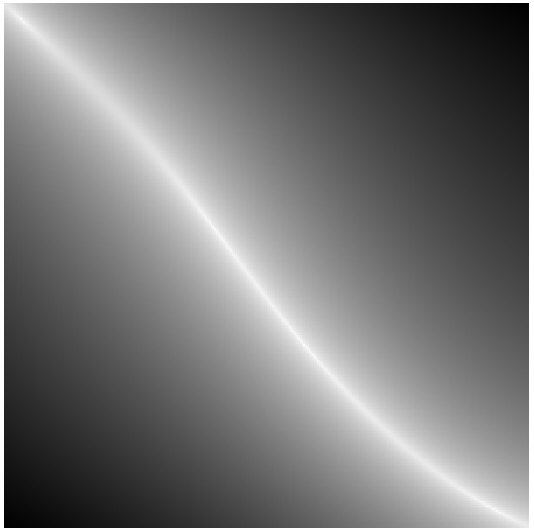
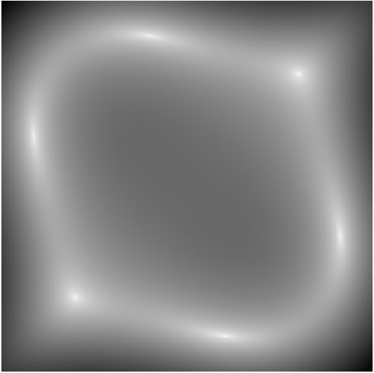
Now here is a plot of the non-linear, two-dimensional distance function between these two curves. The horizontal axis of the plot is the t parameter (time) on one curve, from 0 (start) to 1 (end); the vertical axis is likewise the time on the other curve. Varying these two parameters produces a two-dimensional area, and the distance between the points on the curves at the associated times creates a three-dimensional surface. This surface is plotted here as an 8-bit gray level, white being zero distance and black being the maximum distance. The solution to the intersection problem is to find the locations of the peaks. Visualize this three-dimensional surface by imagining the whitest areas to be mountain peaks, and the darkest areas to be the lowest elevations. Observe the "mountain ridge" which runs from northwest to southeast; this shows how the curves are close together at approximately opposing times, since they run in opposite directions. The four points of intersection are white peaks along this ridge, two close to the ends, and two slightly off from the center. (Your browser may exhibit visible steps in the gray levels and ragged edges on these steps; this is an artifact of the JPEG compression applied to the images.)
Here is the same distance function, except plotted as equidistant contours. This gives a better sense of where the surface peaks are located, since you can see islands at the corners. The long, skinny island in the center has peaks near its ends.
Here is the distance-surface plot for the two pretzel curves. The general shape of the closeness is a mountain ridge that looks like an open mouth. This ridge has six pointy peaks corresponding to the six incisive intersections. The plot is symmetric because the curves are perfectly symmetric mirror images of each other.
Here is the contour version of the distance-surface. It clearly shows the six pointy peaks.
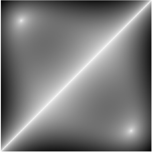
Here is another distance plot of one of the pretzel curves with itself instead of with the other curve, which we call the self-distance-surface. The sharply pointed peaks in the northwest and southeast corners represent the self-intersection of the curve.
Self-distance-surfaces always have (1) a perfectly straight ridge from southwest to northeast, since the comparative times are the same there, and the distance of any point to itself is zero. (2) a symmetry along this same diagonal, resulting in two equal triangular surfaces.
Here is the contour plot of the self-distance surface. It shows the two pointy peaks of self-intersection.
Finding intersections amounts to finding the peaks in these three-dimensional distance-function surfaces. Any algorithm to find intersections will have to map the entire surface, which is intractible if this means evaluating each point on the surface.
However, a bisection algorithm can locate the peaks more efficiently, because it is able to discard large, rectangular areas of the surface as "peakless". It does this by quickly examining the convex hulls of the curves over whole intervals of time, and discarding the intervals from further consideration when the convex hulls do not overlap. For practical computation, this method can take advantage of several convenient properties: (1) that the rectangular bounding box of a Bezier curve is a pessimistic approximation to the curve's convex hull, (2) that this rectangular bounding box is easily found by taking the minima and maxima of the curve's endpoint and control point coordinates, and (3) that overlap of two such rectangles is easily tested by comparing half-planes.
However, bisection starts to fail when peaks become "flat". As the peaks get flatter, areas must be mapped instead of discarded. Peaks become flat whenever curves approach each other in a grazing fashion, instead of incisively. For any convergence criterion we might choose as "close enough" for the bisection algorithm to consider an intersection as having been found, we can always construct a case of two curves that travel together so closely over some shared interval that they appear "close enough" not just at one point but over the whole interval. In visual terms, the bisection algorithm must, of numerical necessity, consider intersection to occur not strictly at the perfect peaks (that is, zero distance), but at any "altitude" above some small distance below the peaks (that is, at some tiny distance of convergence). As peaks flatten, they stop being nice and pointy, and turn into "swamps."
Bisection, in such cases, will truly be "swamped". Instead of reporting such a peak once, bisection will report the intersection many times as it slowly maps the area of the swamp. Such multiple reports cannot be resolved by simply observing their closeness, because truly distinct peaks can be arbitrarily close together.
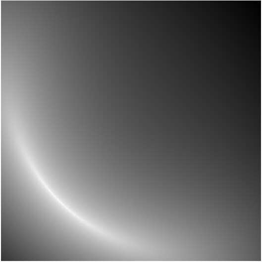
Here is a final example that exhibits such a swamp. Two closed paths graze and just barely cross over, specifically where curves d-c and h-g meet, roughly in the middle of the figure. (The resolution of the diagram is not sufficient to show the dual crossings.)
The distance-surface plot shows a crescent-shaped ridge where the curves approach and cross over. The two crossing points result in two peaks, which are at distinct but close positions near the middle of the crescent. Again, the resolution of the diagram is not sufficient to visibly separate the dual peaks.
(The curves are really the same, one being a translated and rotated copy of the other, so there is some apparent symmetry to this distance-surface.)
The contour plot shows the crescent, but again it does not visually resolve the dual peaks.
Although the crescent ridge contains two true peaks, a long region of it is within the ostensible convergence criterion of a bisection algorithm. Consequently, such an algorithm will not be able to distinguish the dual peaks of the two true intersections, and moreover, will erroneously report that the curves intersect all over some substantial region of this crescent.
The gray-scale distance-surface diagrams bear a remarkable resemblance to astronomical images, and the limits of optical resolution in a telescope are much like our problems of intersection-finding in hard cases. But in our mathematical universe, we do not suffer the limits of building physical instruments of limited size.
So if "there are no good, general methods for solving systems of more than one nonlinear equation," then what hope do we have in this matter of Bezier intersection? The key is to recognize that we need a good, specific (as opposed to general) method, specific to the Bezier equations. Indeed, there is another algorithm altogether, which avoids the inherent numerical confusion of bisection, and which allows us to find the peaks, no more and no less. I am not going to reveal that unpublished algorithm here, but I will give you a hint: one avoids the mire of a swamp by reformulating it as a large set of problems that have a small number of fast, closed-form solutions.
Here are my "torture test" pairs of Bezier curves for those interested in data for their own experimentation:
1.0 1.5 moveto 15.5 0.5 -8.0 3.5 5.0 1.5 curveto
4.0 0.5 moveto 5.0 15.0 2.0 -8.5 4.0 4.5 curveto

664.00168 0 moveto 726.11545 124.22757 736.89069 267.89743 694.0017 400.0002 curveto
850.66843 115.55563 moveto 728.515 115.55563 725.21347 275.15309 694.0017 400.0002 curveto

1 1 moveto 12.5 6.5 -4 6.5 7.5 1 curveto
1 6.5 moveto 12.5 1 -4 1 7.5 6 curveto

315.748 312.84 moveto 312.644 318.134 305.836 319.909 300.542 316.804 curveto
317.122 309.05 moveto 316.112 315.102 310.385 319.19 304.332 318.179 curveto

1046.604051 172.937967 moveto 1046.604051 178.9763059 1041.76745 183.9279165 1035.703842 184.0432409 curveto
1046.452235 174.7640504 moveto 1045.544872 180.1973817 1040.837966 184.0469882 1035.505925 184.0469882 curveto

0uf0d0d1ca63075a40 0u9408ce996a237740 moveto
0u6d5675460fbe5e40 0u6ef501e1b7487940
0u9a71d2f8143d6540 0u6bc18bbe02907a40
0u5b94d92093aa6b40 0u6ac18bbe02907a40 curveto
0u92c56ed7b6145d40 0uede4f1255edb7740 moveto
0u1138c1101af75940 0u42e4f1255edb7740
0u408e51603ad95640 0u1e2e8fe9dd927740
0u1cb4777cd3a75440 0u212e1390de017740 curveto

125.79356 199.57382 moveto 51.16556 128.93575 87.494 16.67848 167.29361 16.67848 curveto
167.29361 55.81876 moveto 100.36128 55.81876 68.64099 145.4755 125.7942 199.57309 curveto
[1] Press, et al., Numerical Recipes in C, 2nd edition, 1992, p. 379.